In certain simple cases, for example when a system includes only one source of waste heat and one single process to be powered, problem of how to insert a heat pump is rather straight forward. However, when it comes to integrating a heat pump with more complex thermal systems, for example a chemical plant or a food processing plant, with many flows to be heated- or to be cooled, the whole thermal network must analysed and optimised in order to recover, where possible, the waste heat through the static exchangers and only after this possibility is fully exhausted, energy from the outside to heat- or cool the remaining loads should be considered. A heat pump can reduce the need for external heating or cooling very substantially when positioned correctly in the optimised thermal system.
The Pinch method was initially developed in the 1970s for the chemical and petrochemical industry, its use has been extended to all energy-intensive sectors (especially the paper industry, food industry and industry steel industry).
This method makes it possible to determine the minimum energy consumption necessary for the operation of a process or an industrial site, the so-called target values. The comparison between these ideal values and the real consumption of the system shows how much energy can be saved by optimizing the exchanger network for heat recovery. The methodology can be applied to each of the site’s energy-intensive processes or to the entire site.
The pinch method allows to analytically design an economically optimal heat exchanger network. In addition, this procedure allows to define the point where to insert the heat pump in the system and the requested temperature levels of the heat source and heat sink.
Here, we limit ourselves to mentioning the main elements of this method. A practical guide to learn more about this topic can be downloaded here.
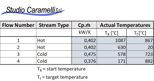
the flow table
Each pinch analysis begins with an inventory of the flows of enthalpy present in the system. For each of them, the starting temperature, the final temperature, the mass flow rate and thermal capacity of the fluid (which is assumed to be constant in the temperature range considered) should be established. In case phase changes occur during the heating or cooling of the fluid, this should be registered as well with the specific change of enthalpy. This data can be derived from measurements of the operational parameters of a process, from simulations or from design data.
Any heat exchangers already present in the system must be excluded. Flows from utilities (boilers, cooling systems, etc.) must also be excluded as well from the table. The figure on the left shows a simple example of such a flow table.
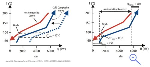
the composite curves
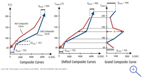
The flow table allows the creation composite curves of the enthalpy flows. A composite curve is a curve that plots for a group of flows, the sum of their enthalpies and the temperatures at which this thermal energy is available. An example of composite curves is shown in the figure on the right. There is a curve that represents the flows that must be cooled (the hot flows, red curve) that have energy to yield and there is a curve of the flows that must be heated (the cold flows, blue curve). The absolute value of enthalpy depends on the choice of the reference level for the enthalpy (h = 0). This implies that you can move the curves on the horizontal axis without altering the information contained therein as shown in figure (a) on the right. Moving the two curves closer to each other, at a certain point they will touch. At this point the temperature difference between the two flow systems is equal to 0 °C. Since in order to have a heat exchange between hot and cold flows, there must be a minimum temperature difference. Therefore, the two curves must be moved to the point where the minimum distance between the two curves is equal to this minimum temperature difference, as can be seen in figure (b).
the optimal heat exchange surface
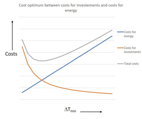
In the area where the two curves overlap, there is the possibility of exchanging heat between the hot and the cold flows. The extreme parts of the curves, without overlap, indicate the minimum demands for heating and cooling, QHmin and QCmin in the figure above. It can be seen from this figure that for a larger ΔTmin, which would correspond to a smaller exchange surface, moving the cold curve to the right, the values of QHmin and QCmin would increase. This means higher external energy consumption. Hence the need to find an optimal point between the investment in the exchange surfaces and the operating costs due to more energy consumption. The optimal value for ΔTmin depends on the shape of the two composite curves, the heat exchange coefficients in the exchangers, the specific cost of energy, the specific cost of the exchangers, etc. A compromise must be reached between the energy saving potential and the corresponding investment amount as illustrated in the figure on the left.
Once the minimum temperature difference is set, the system optimisation consists of coupling the hot and cold flows through heat exchangers in order to transfer the maximum amount of heat between the two flows. If the coupling is perfect (for example without economic or physical constraints), all the heat potentially transferable between the cold composite flow and the hot composite flow will be transferred between the two and the need for external utility (heating or cooling) will be equal to the theoretical minimum. These minimum requirements must be met by external sources (heat generators or coolers).
the pinch
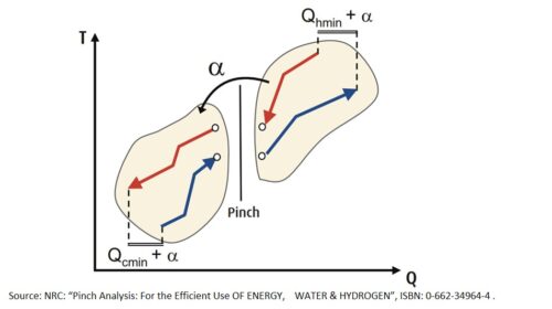
The point where the distance between the two composite curves is minimal, is the point where the ∆Tmin is reached. This is known as the Pinch point. The area above this temperature is the area where there is a net need for thermal energy while in the area below there is a net need for cooling (see figure at the right).
It can be shown that for an optimal system:
external cooling must not be used for flows which are above the Pinch temperature,
external heating must not be used for flows that are below the Pinch temperature and,
heat must not be exchanged across the Pinch, i.e. from a flow with a temperature above the Pinch point towards a flow with a temperature below the Pinch point, or vice versa (indicated as α in the figure on the right).
These are the three fundamental rules of the Pinch Analysis.
the Grand Composite Curve
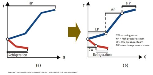
Most processes are heated and cooled using different temperature levels for the external utilities (for example: steam at different pressure levels, cooling water, chilled water, etc.). Generally speaking, the cost of thermal energy increases when its temperature increases (note: the opposite is true for cooling). This cost increase is particularly significant when thermal energy is produced with a heat pump or with a solar thermal system. To minimize the costs for energy, each process must be fired with the cheapest utility possible. For example, it is preferable to use low pressure steam rather than high pressure steam and cooling water rather than using a refrigeration system.
Although composite curves provide the overall energy targets, they do not give us any indication of how much energy needs to be brought into the process (or subtracted from the process) at which temperature. The tool for obtaining this information is the Grand Composite Curve (see the figure on the left).
how to use the grand composite curve
The Grand Composite Curve shows, at each temperature level, the difference between the hot- and cold composite curve, as illustrated in the figure above. The shifted composite curves are created by moving the hot composite curve 1/2 ∆Tmin degrees down, and the cold composite curve 1/2 ∆Tmin degrees up. So they will touch at the Pinch point. The figure on the right illustrates how with the help of the Grand Composite Curve it is possible to find the quantities and the relative temperatures of the external energy that should be supplied in order to meet the energy needs of this specific process.
In summary, the Grand Composite Curve is the basic tools used in the Pinch Analysis used to visualise the temperature levels of the external energy to be supplied to a process as function of the temperature level.
how to integrate a heatpump
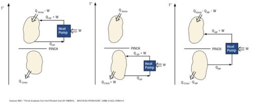
If evaporator and the condenser of the heat pump is are both connected to flows above the Pinch, case (a) in the figure on the left, it simply transforms electrical energy used by the compressor into heat. This because the evaporator of the heat pump subtracts heat above the Pinch where no cooling is needed. Of course, this is not useful. If the heat pump is positioned completely below the pinch, the case (b) in the figure, the situation is even worse since no heat is needed below the Pinch. The electricity for the compressor is transformed into waste heat which increases the need for external cooling (cold utility).
The only appropriate way to position a heat pump is to place the evaporator below the Pinch and the condenser above, case (c). In this case, heat is absorbed below the Pinch so the need for cooling decreases and the heat from the heat pump is delivered above the Pinch so the need for hot utility is reduced by the same amount.
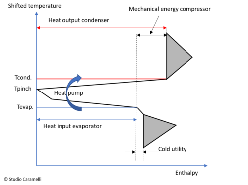
a heat pump in the grand coposite curve
The figure on the right shows a Grand Composite Curve with a heat pump. The curve indicates at what temperature the heat pump must supply the thermal energy to the system (Tcond.) And at what temperature there is heat available for the evaporator. From the curve it can be seen that in this case the hot utility is 100% covered by the energy supplied by the condenser. The cold utility is almost entirely covered by the evaporator.
The shape of the curve indicates whether the thermal system is suitable for inserting a heat pump or not. If the Pinch is very narrow, or sharp, around the pinch point (as in the figure), so the lines starting from the Pinch are almost horizontal, then the temperature difference between the evaporator and the condenser will be low, which is favourable for the COP. A wider curve leads, with the same amount of energy supplied by the heat pump, to a larger temperature difference between the evaporator and the condenser and as a consequence, to a lower COP.